|
|
|
In the 17th century, Sir Isaac Newton, in an attempt to study the orbits of the planets in our solar system, discovered that his equations of motion weren't able to accurately predict the orbits of our celestial bodies. He realized that gravitational forces between all the planets would influence their orbits, and thus the n-body problem was born. The n-body problem is an interesting and complex topic that can be used to study the dynamics of heavenly bodies as well as other particle interactions, such as particles in an electric field. We were inspired by this problem to create a simulator that models the interaction of particles in space under the influence of gravitational forces.
Our technical approach involves developing a gravity particle simulator that simulates the interactions of particles in a gravitational field. We decided to use Cloth Sim as a skeleton and general architecture for our N-Body Sim because we wanted to make use of the camera, GUI, and renderer methods. To improve the performance when simulating a large number of particles, we used the Barnes-Hut algorithm, which reduces the computational complexity of simulating N-bodies from $O(N^2)$ to $O(N\log{N})$ by grouping particles into an octree. We also added a few new shaders to add visual flair to our particles and improved upon the GUI to add features that allow for dynamically creating different particle configurations, setting simulation speeds, and swapping shaders.
Our first objective was to understand the Cloth Sim pipeline and GUI / program initialization so we could clone a skeleton version of it. This involved reading clothSimulator.h/cpp and main.cpp to understand how the GUI, renderer, and camera were initialized and being used. Once we had a general understanding, we created a new CMAKE project and copied over the code for any relevant methods, removing unused parameters and objects. After we got our project to compile, our next objective was to render a few spheres. In Cloth Sim, we don't render any point masses, only the wireframe that's attached to each Spring. For our purposes, we wanted to render particles as spheres, so we used SphereMesh::draw_sphere(), which would render a sphere of specified position and size with a shader applied to it. This ended up being perfect for our use case, so we created a new Particle class that would call this method when Particle::render(GLShader) was called on it. This allowed us to successfully render a few particles on the GUI.
In each step of our simulate method, we compute the forces on each particle and then update the position and velocity for every particle. Interactions between particles in space are determined by Newton's Law of Universal Gravitation, which states:
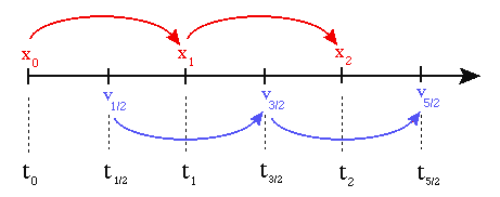
When updating the positions of the particles, we used numerical integration to estimate the position and velocity at the next timestep. Initially, we used Forward Euler, a first-order, explicit numerical integrator, to test if our system could run with a few particles. The Forward Euler update rule is defined as such:
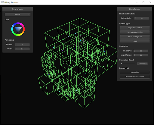
In order to compute the net force on each particle, we initially ran a quadratic algorithm to compute the pairwise force between all the particles. As one might imagine, for large number of particles (1000+) our simulation begins to significantly slow down. The primary optimization approach we took was to adopt the Barnes-Hut algorithm. This algorithm allowed us to reduce the runtime to compute forces on the particles from $O(N^2)$ to $O(NlogN)$. There are two phases to this algorithm: (1) building the octree out of the particles, and (2) computing the forces on each particle using the octree. We will refer to the octree in Barnes-Hut as a BHTree from now on.
In a BHTree, only the external nodes contain either a single particle or no particles. The internal nodes on the other hand contain no particles but store the center of mass as well as the total mass of all the particles contained within its subtree. When computing the net force on a particle, if the center of mass of the octant the particle is sufficiently far, then we approximate all of the particles in that octant as a single particle such that its total mass is equal to the sum of all the masses of the particles in it. Below is the condition that determines whether or not the center of mass of an octant is sufficiently far:
Where $d$ is the distance between the particle and the center of mass of the octant, $L$ is the length of the diagonal of the octant's bounding box, $\delta$ is the distance between the octant's geometric center and the its center of mass. Finally, $\theta$ is a parameter we chose that essentially dictates the "leniency" of the approximation. Low $\theta$ values increase the accuracy of the force computations but slow the algorithm down ($\theta = 0$ is equivalent to naive), and high $\theta$ values decrease the accuracy of the force computations but speed up the algorithm (more approximations occur). After some tuning, we decided to use $\theta = 0.7$.
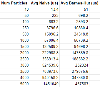
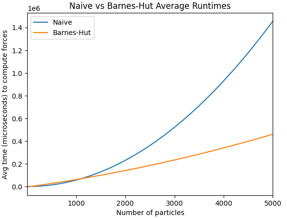
Below are some runtime statistics displaying how Barnes-Hut outperforms Naive solution for large number of particles. Computer specs:
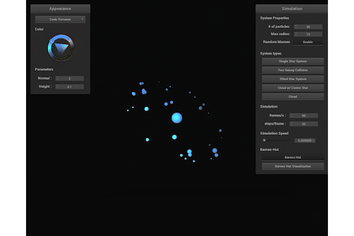
Once the simulation logic was implemented, we wanted an easy way to create interesting simulations. For example, we have simulations for a single galaxy, two galaxies colliding, a particle cloud with no central star, and more. Each simulation has a button in the GUI that you can click to switch between. To start playing the simulation press 'P' and press 'P' again to pause it. To restart the simulation or update any changed configurations, press 'R'. There is also a button that toggles a feature to randomize the masses of the particles. Just like Cloth Sim, there's also a way to change the shaders applied to the spheres. There's also a slider to speed up the simulation by multiply the timestep $\Delta t$ by a factor from $0.0$ to $100.0$.
When we're generating particles, we use the sampler.cpp class from Pathtracer, specifically UniformSphereSampler. This function allows us to generate a uniform distribution of particles with various configurations. For example, by default we only use the $x, y$ components and vary the $z$ component to be some random constant between -2 and 2. We can easily multiply the output from the sampler by a constant to achieve any max radial distance we desire. If we want to create a tilted galaxy, we can project the sampled point onto a plane that intersects the sphere. We can do this simply by defining a point on the plane $P$ to be the center of the sampled sphere, and defining the normal of the plane to be some arbitrary unit vector $\hat{n}$. We can then use a the ray-plane intersection to project the sampled point on the surface of the sphere directly onto the plane using its $\hat{n}$. We used a combination of these methods to create different "star systems".
Initially, we actually struggled with creating "space-like" simulations because of the fact that when a simulation starts, particles would simply be attracted directly towards the center star instead of orbiting it. To address this, we gave each particle an initial tangential velocity, and this was sufficient to allow particles to orbit in a more realistic fashion. We calculated the tangential velocities by performing the following calculations. We define the center star to be position $\vec{p_0}$ and mass $M$ and each particle has a position $\vec{p}$ and mass $m$. The galactic plane is defined to have a unit normal $\hat{n}$, for a non tilted system, the galacic normal is $(0, 1, 0)$. The tangential velocity direction $\vec{v_t} = (\vec{p} - \vec{p_0}) \times n$. The magnitude of velocity uses the centripetal acceleration formula $a_c = v_t^2 / r$, where $a_c = GM / r^2$, solving for $v_t$ gives $\vec{v_t} = \sqrt{\dfrac{GM}{r}} \hat{v_t}$.
We also multiply all initial velocities with a dampening factor $10^{-4}$ which was chosen based off experimentation to prevent masses from accelerating too fast out of orbit. This was also necessary because the distances between our particles were very small compared to their masses, which meant we had to scale up the distances when performing force calculations, and dampen inital velocities. While this simply the easiest solution, its possible to define an optimization problem or machine learning algorithm to determine good inital values in such a way that the particles don't accelerate too quickly and immediately get flung out of orbit. This would be something we could expand upon in the future.
During our research, we wanted to find different rendering models compared to those we've seen in lecture. This is how we stumbled upon the Cook-Torrance model. The Cook-Torrance model is a microfacet model used for simulating the appearnce of rough surfaces. It uses a combination of the surface roughness and the surface reflectance to calculate its appearance. It is widely used to simulate metals, plastics, and ceramics, but we thought it would be itneresting to try to implement.
The equation for the Cook-Torrance model is
Where $f_{lambert}$ is the diffuse component, and $f_{cook_torrance}$ is the specular component. Instead of $k_d$ and $k_s$, we used a single variable $s$ to represent the ratio of light diffused and specularly reflected, changing our equation to
The diffuse component is the same as that of the Phong model: $f_{lambert} = (I/r^2) max(0, n \cdot l) $u_{color}$, which is the color chosen from the GUI, acting as the diffuse coefficient. The specular component, however, has the following function as its specular coefficient:
The distribution function $D$ is the part of the Cook-Torrance model that describes the concentration of microfacets oriented to reflect specularity. There are many choices of functions that can be used to describe this distribution, so we chose to use the Phong distribution to keep results close to something we are famiilar with:
Here, $\alpha$ represents the roughness of the object. We used $\alpha = 0.6$ because it gave the best appearance given the position of our light source and the distribution of particles.
The geometry function $G$ is used to describe the proportion of light that the microfacets do not block by either occludding or shadowing each other. Therefore, it is defined as the minimum of two different factors calculating either type of attenuation.
Finally, the fresnel function $F$ is used to simulate the way light itneracts with a surface at different angles. The equation for $F$ changes depending on whether the material is a dielectric or a conductor. Because a particle wouldn't necessarily be a dielectric or conductor type of material, we used Schlick's Approximation, as it allows us to approximate the fresnel function considering both materials properties:
Here $F_0$ is the reflectance at normal incidence, and $n$ is the material's index of refraction. We chose an arbitrary $n$ of $n = 1.2$.
The intention of the Planet shaders were to color the particle by useing noise to randomly sample its surface. We used the position of a given particle as the input to our noise function, causing the smaller particle to appear as if they had their own spin as they orbits around a large mass in our simulations. While trying various combinations of functions to declare the color at a given pixel in the shader, we stumbled upon the result of what can be described as "sun flares" on our particles, long stripes across the surface of the particle that seem to merge and diverge from each other seemingly at random.
Overall, this project was a very fun and rewarding experience. We learned a lot more details about CMAKE and OpenGL such as compiling projects and dependencies and deepened our understanding of the OpenGL pipeline. We also learned a lot more about the N-body problem and its different applications by reading research papers of various applications and techniques. We learned about the Barnes Hut algorithm and worked with an octree for the first time. When creating shaders, we learned new methods that weren't covered in class, such as random noise generation. Most importantly, we learned that realistic physical simulations are hard!
There were many issues that we encountered, such as incorrect mass and distance ratios that would cause our simulation to have undesired behavior. We focused more on using Newton's laws to produce nice looking results, as we based our mass ratios off of the Sun to Earth masses, and scaled our distances and dampened velocities so that they would look good. In reality, celestial bodies have a huge range of masses and the distances between them are truly astronomical. The time scales are also impossible to simulate in "real time", otherwise we'd have to wait a year for an Earth-like mass to orbit around a Sun-like star. Futhermore, many realistic galatic simulations must take into account the effects of dark matter and general relativity. Additionally, other simulations that we've researched seem to render hundreds of thousands of particles as pixels, whereas we rendered them as spheres. Because of our rendering method, we weren't able to render over a couple hundred particles without experience serious slowdowns. However, if we wanted to simulate a large number of particles, we had a solution for this: render a few thousand particles with laggy simulation footage, and use frame interpolation to speed it up in post production (this was done in Adobe Premiere Pro). We used this method to produce the cinematic at the beginning of the final video.
Despite all this, we believe we had successfully implemented an N-body simulation that models the behavior of celestial bodies. We set out with a goal to produce semi-realistic behavior of colliding galaxies in space, and our simulation works well for up to a few hundred particles, and we used our frame interpolation method to create cool visuals.